Powering the minimum-effect claim • powerape

Why power for an APE at all?

In a probit or logit model, the coefficient is not the quantity anyone interprets. Applied conclusions are stated in probability points – “the treatment raises take-up by 10 percentage points” – which is the average partial effect (APE). The APE depends on all coefficients and on the covariate distribution, so power tools that work in coefficient or Cohen’s-d units cannot answer the question practitioners actually have.

powerape lets you specify the target in APE units and simulates the whole pipeline: draw covariates, draw outcomes, fit the model by maximum likelihood, compute the APE with a delta-method Wald confidence interval, and evaluate a claim on that interval (Riesthuis, 2024):

"minimum" – the CI lower bound exceeds the smallest effect size of interest (SESOI): the effect is meaningfully large. This is the default claim and the package’s reason to exist.
"detect" – the CI excludes zero (directional).
"equivalence" – the CI lies inside (-SESOI, +SESOI): the effect is too small to matter.

The Stata command powerape takes the same six steps in the same world: see Get started in Stata.

Step 1: describe the world

library(powerape)

d <- ape_dgp(
  model       = "probit",
  focal       = pa_var("treat", "binary", p = 0.5),
  covariates  = list(pa_var("age", "normal", mean = 45, sd = 12),
                     pa_var("female", "binary", p = 0.55)),
  correlation = 0.2,
  baseline    = 0.30,   # P(Y = 1) with treat = 0
  signal      = 0.15    # latent pseudo-R2 of the covariates
)

The nuisance side is anchored on a friendly scale: the baseline outcome rate and the covariates’ latent pseudo-R-squared. Explicit coefficients (gamma), pilot data (ape_dgp_empirical()), or a fitted pilot model (ape_dgp_from_fit()) are the expert routes. The signal fixes the latent error variance at 1, which is exact for probit; under model = "logit", whose latent error variance is pi^2/3, the same signal is a weaker world, and ?ape_dgp gives the conversion from a logit pilot’s McKelvey-Zavoina R-squared.

Step 2: pin the true APE (the inversion step)

Suppose theory or prior evidence suggests a true effect of 10 percentage points, and effects below 5 points would not justify the intervention: the planning value is 0.10 and the SESOI is 0.05.

d <- set_ape(d, target = 0.10)
d
#> powerape DGP -- probit
#>   focal: treat (binary, p = 0.50)
#>   covariates: age (normal, mean 45.00, sd 12.00), female (binary, p = 0.55) 
#>   baseline P(Y=1 | reference) = 0.300, nuisance signal (latent pseudo-R2) = 0.150
#>   true APE pinned at +0.1000 (beta_focal = 0.2943, implied P(Y=1 | focal=1) = 0.400)

set_ape() solves for the focal coefficient that makes the true APE exactly 0.10 given everything else, and errors informatively if the target is infeasible (an APE of +0.40 cannot exist at a baseline rate of 0.85).

Step 3: power for the claim

ape_power(d, n = 1500, claim = "minimum", sesoi = 0.05,
          nsim = 500, seed = 1)
#> powerape -- minimum-effect claim (CI lower bound > 0.050)
#>   probit, n = 1500, assumed true APE +0.1000, 90% CI (alpha = 0.05), nsim = 500
#>   power = 0.656 (MCSE 0.021)
#>   outcomes: minimum 0.656 | detect-only 0.336 | inconclusive 0.008 | equivalence 0.000 | failed 0.000

Read the outcome distribution, not just the power number: some studies would reject zero yet remain unable to claim the effect clears the SESOI (“detect-only”) – exactly the inconclusiveness Riesthuis (2024) warns about.

Step 4: required sample size and the power curve

ape_n(d, power = 0.80, claim = "minimum", sesoi = 0.05,
      nsim = 500, seed = 2)
#> powerape required sample size -- minimum claim
#>   n = 2106 for 80% target power (confirmed 0.806, MCSE 0.009)
#>   assumed true APE +0.1000, sesoi 0.050, 90% CI (alpha = 0.05), probit
#>   search: 1 step(s); confirmed in 1 round(s) at nsim = 2000.

cv <- ape_curve(d, n = seq(500, 3000, by = 500), claim = "minimum",
                sesoi = 0.05, nsim = 300, seed = 3)
plot(cv, target_power = 0.80)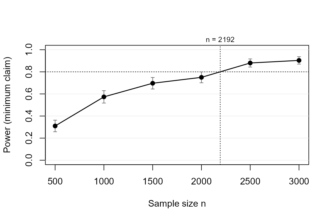

When n is fixed: the minimum detectable effect

Often the design question runs the other way: the archive has the firms it has, and the honest question is what the study can find, not what it would need. ape_mde() inverts the search — the world and the claim stay fixed, and the smallest effect that reaches the target power is solved for, with the same conservative confirmation stage as ape_n() (pushed upward, never down, when the high-precision run falls short):

ape_mde(d, n = 1500, claim = "minimum", sesoi = 0.05,
        nsim = 500, seed = 6)
#> powerape minimum detectable APE -- minimum claim
#>   MDE = 0.1094 at n = 1500 for 80% target power (confirmed 0.811, MCSE 0.009)
#>   smallest effect demonstrably above sesoi 0.050
#>   search: 1 step(s); confirmed in 1 round(s) at nsim = 2000.

If the answer is larger than any effect you would defend as plausible, the design cannot support the study — knowable before the data are touched. The contextual guesses matter here too: ape_robust(mode = "mde") reports the minimum detectable effect per scenario, with the largest MDE as the worst case.

Step 5: how fragile is this to the contextual guesses?

The baseline rate and the covariate signal are guesses, and power computed from a single guess is fragile (Hancock & Feng, 2026). ape_robust() re-runs the analysis over a scenario grid and reports the worst case; with nmax = TRUE it also finds n_max, the insurance-premium sample size: the largest requirement across the scenarios, at nmax_power (90% by default, the default of ape_n(); pass nmax_power = 0.80 for the conventional target).

ape_robust(d, n = 2200, claim = "minimum", sesoi = 0.05,
           vary = list(baseline = c(0.20, 0.40)), grid_points = 3,
           nsim = 300, seed = 4, nmax = FALSE)
#> powerape robustness sweep -- minimum claim, APE, pin = ape
#>   n = 2200, nsim = 300 per scenario, 3 scenario(s) over: baseline
#>   power range [0.797, 0.847]; worst scenario:
#>  baseline implied_effect     power      mcse separated
#>       0.4            0.1 0.7966667 0.0232371         0
#>   scenarios:
#>  baseline implied_effect     power       mcse separated
#>       0.2            0.1 0.8466667 0.02080242         0
#>       0.3            0.1 0.8466667 0.02080242         0
#>       0.4            0.1 0.7966667 0.02323710         0

By default the APE is re-pinned in every scenario (pin = "ape"), so only the precision channel varies; pin = "coefficients" instead holds the coefficients and lets the implied effect drift.

Step 6: the citable paragraph

pw <- ape_power(d, n = 2200, claim = "minimum", sesoi = 0.05,
                nsim = 500, seed = 5)
power_statement(pw)
#> We conducted a simulation-based power analysis for the average partial effect
#> (APE) of treat using the powerape package (version 1.11.4), following the
#> confidence-interval approach of Riesthuis (2024). The assumed data-generating
#> process was a probit model with focal variable treat (binary, prevalence
#> 0.50); parametric covariates age (continuous, mean 45, SD 12), female
#> (binary, prevalence 0.55), with an exchangeable latent (Gaussian-copula)
#> correlation of 0.20 among the focal variable and the covariates; baseline
#> outcome rate 0.300 with the focal at reference; nuisance covariates
#> contribute a latent pseudo-R-squared of 0.15. The assumed true APE was 0.100
#> (10.0 percentage points). At a sample size of n = 2200, simulated power for
#> the minimum-effect claim (the 90% confidence interval's lower bound exceeding
#> the smallest effect size of interest, 0.050; a one-sided test at alpha = 5%)
#> was 0.808 (Monte Carlo SE 0.018; 500 replications). Across replications, the
#> probability of concluding a meaningful effect was 0.808, of detection without
#> meaningfulness 0.192, of an inconclusive result 0.000, and of equivalence
#> 0.000. Estimation used maximum likelihood with delta-method Wald confidence
#> intervals; replications without a maximum-likelihood estimate, from a failed
#> fit or from separation (a focal cell with no events or no non-events),
#> counted against the claim (0.0% of replications).

References

Hancock, G. R., & Feng, Y. (2026). nmax and the quest to restore caution, integrity, and practicality to the sample size planning process. Psychological Methods, 31(1), 174-199.
Riesthuis, P. (2024). Simulation-based power analyses for the smallest effect size of interest: A confidence-interval approach for minimum-effect and equivalence testing. AMPPS, 7(2).