Creates a plot of alpha as function of sample size for the chosen methods
Source:R/alphaN_plot.R
alphaN_plot.RdDraws alpha as a decreasing function of the sample size for any selection
of the calibration methods offered by alphaN(). The prior-fraction
curves ("JAB", "min", "robust", "balanced") are evaluated exactly at every
sample size; the "ES" and "moment" curves are evaluated at twelve
log-spaced sample sizes and interpolated by a spline on the log-log
scale, which keeps the plot fast (expect roughly a second of computation
per Klauer-type curve). Colors follow the colorblind-safe Okabe-Ito
palette.
Usage
alphaN_plot(
  BF = 1,
  max = 10000,
  ylim = NULL,
  methods = c("JAB", "min", "robust", "balanced"),
  de = 0.5,
  log = ""
)
Arguments
- BF
Bayes factor you would like to match. 1 to avoid Lindley's Paradox, 3 to achieve moderate evidence and 10 to achieve strong evidence.
- max
The maximum number of sample size. Defaults to 10,000.
- ylim
Limits for the y-axis. The default, NULL, covers all requested curves. Set to e.g. c(0, 0.05) to zoom in on small alpha levels.
- methods
Character vector with the methods to draw, any subset of c("JAB", "min", "robust", "balanced", "ES", "moment"). Defaults to the four prior-fraction methods, matching the behavior of earlier package versions.
- de
The prespecified (targeted) effect size in standardized units: Cohen's d for
q = 1and Cohen's f for joint tests (the scales coincide atq = 1). Only used by methods "ES" and "moment". Defaults to 0.5, a medium effect; use 0.2 for small and 0.8 for large effects (Cohen, 1988).- log
Passed to
plot(): "" (default) for linear axes, "x", "y", or "xy" for logarithmic ones. Logarithmic axes are useful when the "moment" curve is included, since it falls much faster than the others.
Examples
# Plot of alpha level as a function of n for a Bayes factor of 3
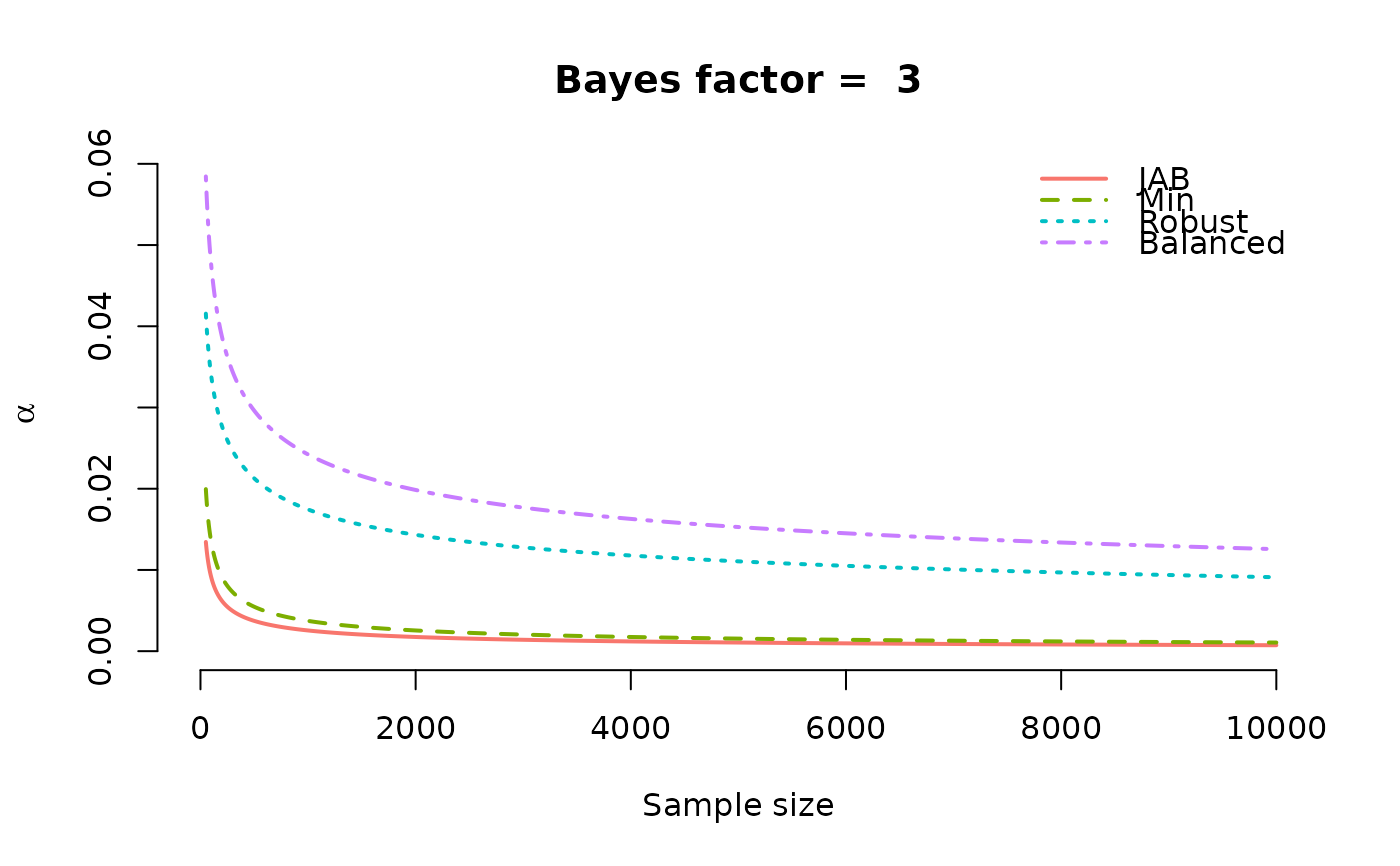
alphaN_plot(BF = 3)
 # Compare JAB with the effect-size and moment calibrations
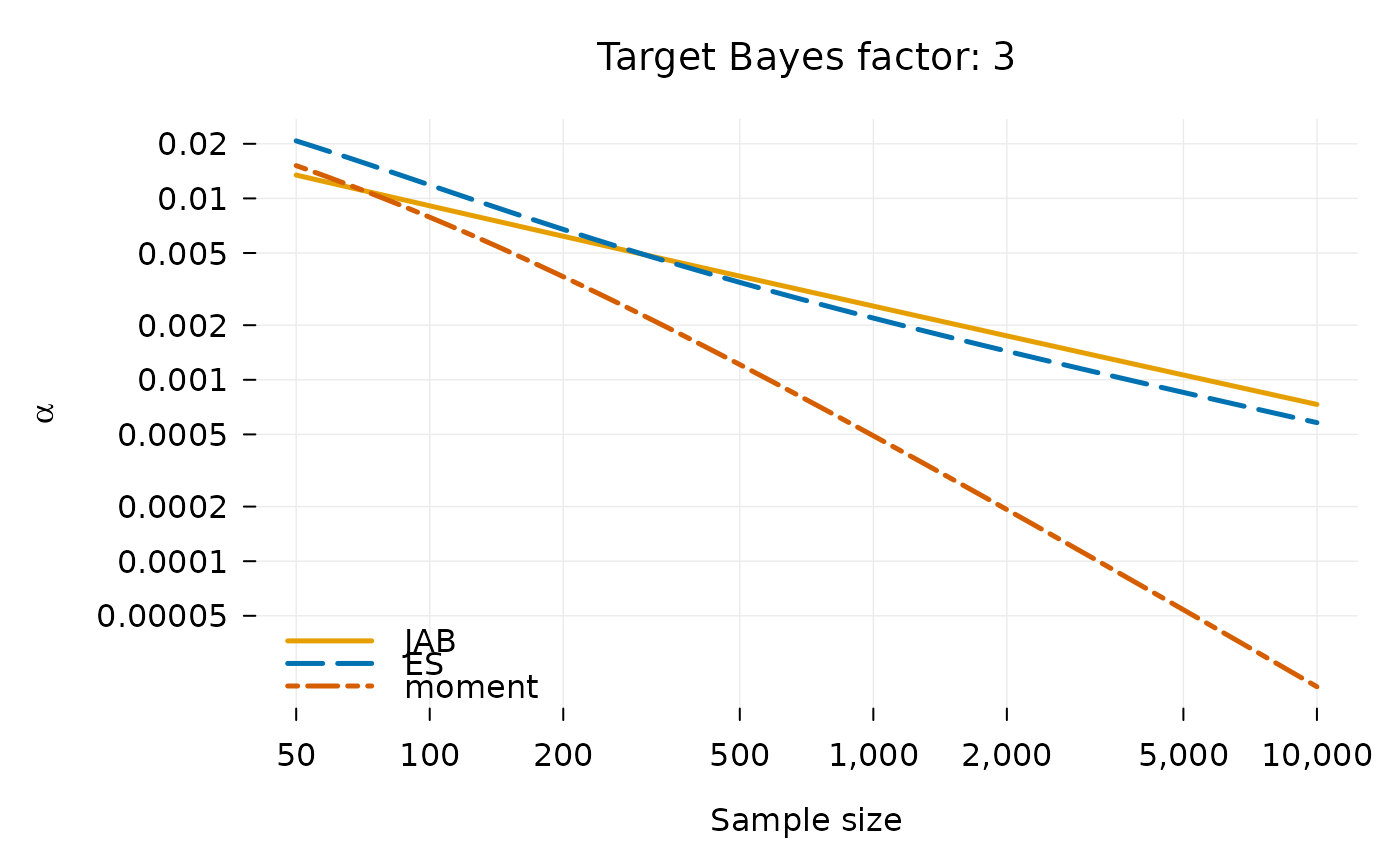
alphaN_plot(BF = 3, methods = c("JAB", "ES", "moment"), log = "xy")
# Compare JAB with the effect-size and moment calibrations
alphaN_plot(BF = 3, methods = c("JAB", "ES", "moment"), log = "xy")