Set the alpha level based on sample size for coefficients in a regression model
Source:R/alphaN.R
alphaN.RdComputes the alpha level required to achieve a desired level of evidence,
expressed as a Bayes factor, when testing a coefficient in a regression
model. The alpha level is a decreasing function of the sample size.
Vectorized over n and BF.
Arguments
- n
Sample size. A positive numeric vector.
- BF
Bayes factor you would like to match. 1 to avoid Lindley's Paradox, 3 to achieve moderate evidence and 10 to achieve strong evidence.
- method
Which Bayes factor to calibrate alpha to. The first four options invert Jeffreys' approximate Bayes factor and differ in the choice of the prior fraction 'b'; the last two invert the exact test-statistic Bayes factors of Klauer et al. (2025), whose priors center the alternative hypothesis on a prespecified effect size
de. One of:"JAB": this choice of b produces Jeffreys' approximate BF (Wagenmakers, 2022)
"min": uses the minimal training sample for the prior (Gu et al., 2018)
"robust": a robust version of "min" that prevents too small b (O'Hagan, 1995)
"balanced": this choice of b balances the type I and type II errors (Gu et al., 2016)
"ES": calibrates alpha to the effect-size Bayes factor (Klauer et al., 2025)
"moment": calibrates alpha to the moment Bayes factor (Klauer et al., 2025), under which effects close to zero are a priori implausible
- upper
The upper limit for the range of realistic effect sizes. Only relevant when method="balanced". Defaults to 1 such that the range of realistic effect sizes is uniformly distributed between 0 and 1, U(0,1). Conceptually,
upperplays for the "balanced" method the role thatdeplays for "ES" and "moment": both declare which effect sizes the researcher deems realistic.uppertreats them as a uniform band whose Type I and Type II error rates are then balanced, whereasdesingles out a focal effect size on which the prior concentrates.- de
The prespecified (targeted) effect size in standardized units: Cohen's d for
q = 1and Cohen's f for joint tests (the scales coincide atq = 1). Only used by methods "ES" and "moment". Defaults to 0.5, a medium effect; use 0.2 for small and 0.8 for large effects (Cohen, 1988).- nu
Degrees of freedom of the prior t distribution for methods "ES" and "moment". The default, NULL, uses the values recommended by Klauer et al. (2025): 3 for "ES" and
5 + (q - 1)for "moment".- r
Scale of the two prior mixture components for method "ES". The default, NULL, uses the recommendation of Klauer et al. (2025),
r = sqrt((nu - 2)/(nu * q)) * de, which requires nu > 2 and de > 0; otherwise supplyrexplicitly.- q
Number of coefficients tested jointly. Only used by methods "ES" and "moment". The default, 1, is the test of a single coefficient; for
q > 1the alpha level is set for the F test of the joint null that all q coefficients are zero.- p
Number of parameters retained in the model under the null, including any intercept. Only used by methods "ES" and "moment". The effective sample size of Klauer et al. (2025) is
n - p; the default, 0, reproduces the one-sample form, which treats the sample size as effective. For a regression coefficient in a small sample, settingpto the number of other estimated coefficients (including the intercept) gives the residual-degrees-of-freedom behavior of the exact regression case.
Details
For methods "ES" and "moment" with q = 1, the alpha level is found by
solving for the critical t value at which the effect-size or moment Bayes
factor equals BF, and converting that critical value to a two-sided
p-value on the t distribution with n - p - 1 degrees of freedom. For
q > 1, the same inversion runs through the noncentral-F form of the
Bayes factors (Klauer et al., 2025, Table 4), and alpha is a p-value on
the F distribution with (q, n - p - q) degrees of freedom. The
implementation is validated against the Bayes factors reported in Tables
7 and 8 of that paper. Because the moment prior assigns effects near zero
a priori density zero, the alpha level it implies decreases much faster
with n than under JAB.
Klauer et al. (2025) derive these Bayes factors under the normal linear
model (t tests, linear regression, ANOVA). For other generalized linear
models, the "ES" and "moment" calibrations hold in the same asymptotic
sense as the prior-fraction methods, whose Wald-based derivation covers
any generalized linear model directly; for non-Gaussian models with
modest n, prefer the prior-fraction methods.
As a special case, setting method = "ES", nu = 1, de = 0 with an
explicit scale (e.g. r = 1) calibrates alpha to the default
(Jeffreys-Zellner-Siow type) Bayes factor of Rouder et al. (2009).
For effective sample sizes greater than 50,000, methods "ES" and "moment" evaluate the noncentral density ratio in its normal (or chi-square) limit, which is accurate to a fraction of a percent there.
References
Gu et al. (2016). Error probabilities in default Bayesian hypothesis testing. Journal of Mathematical Psychology, 72, 130–143.
Gu et al. (2018). Approximated adjusted fractional Bayes factors: A general method for testing informative hypotheses. The British Journal of Mathematical and Statistical Psychology, 71(2).
Klauer, K. C., Meyer-Grant, C. G., & Kellen, D. (2025). On Bayes factors for hypothesis tests. Psychonomic Bulletin & Review, 32, 1070–1094. doi:10.3758/s13423-024-02612-2
O’Hagan, A. (1995). Fractional Bayes Factors for Model Comparison. Journal of the Royal Statistical Society. Series B (Methodological), 57(1), 99–138.
Rouder, J. N., Speckman, P. L., Sun, D., Morey, R. D., & Iverson, G. (2009). Bayesian t tests for accepting and rejecting the null hypothesis. Psychonomic Bulletin & Review, 16, 225–237.
Wagenmakers, E.-J. (2022). Approximate objective Bayes factors from p-values and sample size: The 3p(sqrt(n)) rule. PsyArXiv.
Wulff, J. N., & Taylor, L. (2024). How and why alpha should depend on sample size: A Bayesian-frequentist compromise for significance testing. Strategic Organization, 22(3), 550–581. doi:10.1177/14761270231214429
Examples
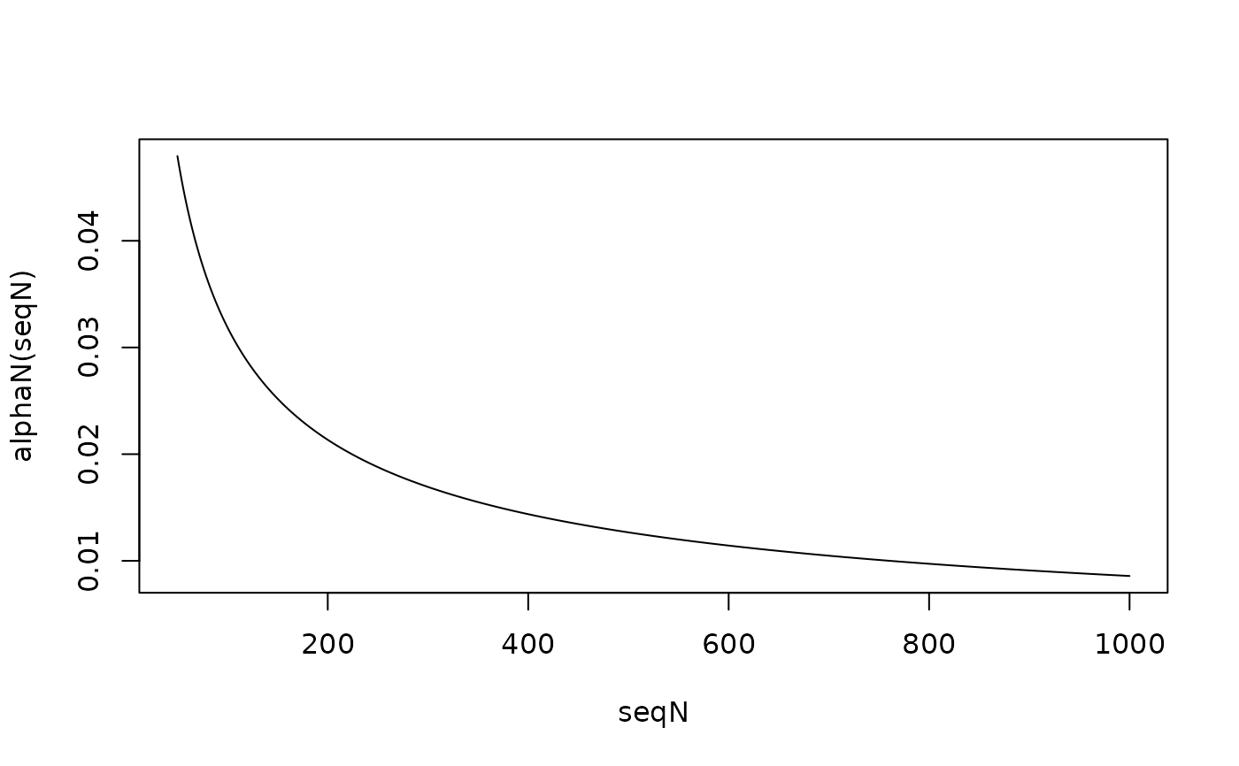
# Plot of alpha level as a function of n
seqN <- seq(50, 1000, 1)
plot(seqN, alphaN(seqN), type = "l")
 # Alpha calibrated to the effect-size Bayes factor (Klauer et al., 2025),
# targeting moderate evidence for a medium-sized effect
alphaN(1000, BF = 3, method = "ES", de = 0.5)
#> [1] 0.002189564
# The same calibration under the moment Bayes factor
alphaN(1000, BF = 3, method = "moment", de = 0.5)
#> [1] 0.0004913521
# Alpha for the joint F test of q = 2 coefficients in a model with an
# intercept and one further retained coefficient (p = 2), targeting a
# medium effect on Cohen's f scale
alphaN(200, BF = 3, method = "ES", q = 2, p = 2, de = sqrt(0.15))
#> [1] 0.008427417
# Alpha calibrated to the effect-size Bayes factor (Klauer et al., 2025),
# targeting moderate evidence for a medium-sized effect
alphaN(1000, BF = 3, method = "ES", de = 0.5)
#> [1] 0.002189564
# The same calibration under the moment Bayes factor
alphaN(1000, BF = 3, method = "moment", de = 0.5)
#> [1] 0.0004913521
# Alpha for the joint F test of q = 2 coefficients in a model with an
# intercept and one further retained coefficient (p = 2), targeting a
# medium effect on Cohen's f scale
alphaN(200, BF = 3, method = "ES", q = 2, p = 2, de = sqrt(0.15))
#> [1] 0.008427417